Monthly Archives: December 2013
Aerofoil (Flowsquare wind tunnel)

Premixed Flame Propagation

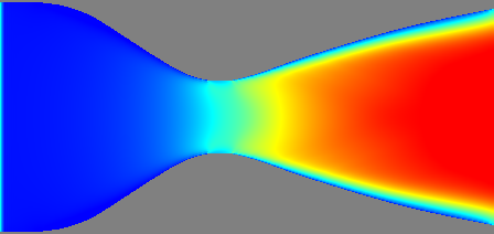
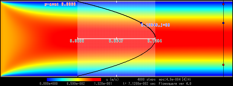
Channel flow (high-order scheme)
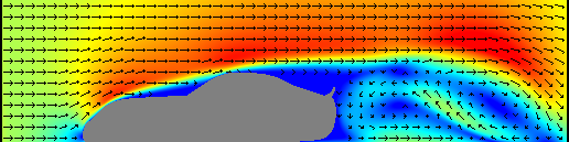
Flow Around a Car
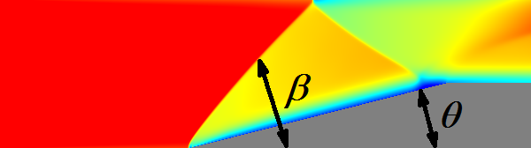
Oblique Shock
Kelvin-Helmholtz Instability

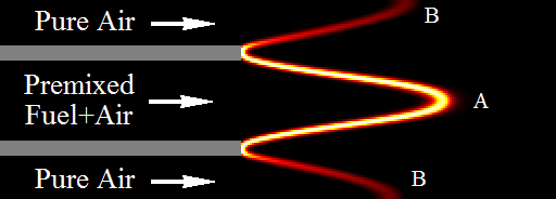
Bunsen Flame
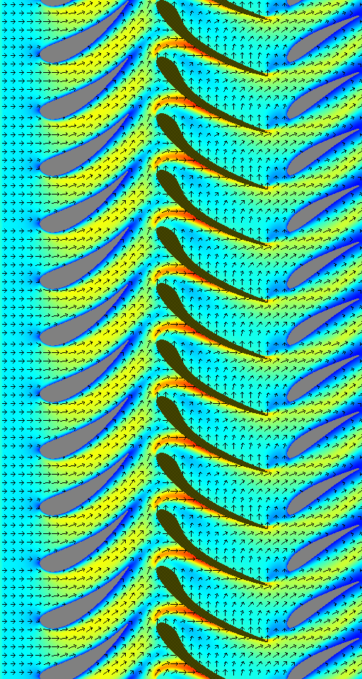
Jet Engine Compressor
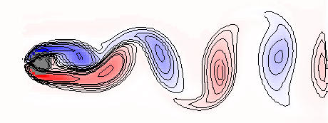
Karman Vortex Street
Lesson 3 — Keyboard shortcut
There are many keyboard shortcuts used in Flowsquare. Note these keyboard operations are detected once in a transition between displays from an old time step (eg. n-1) to a new time step (eg. n), and the operation is reflected in display for the next time step (eg. n+1). Continue reading
Lesson 2.3 — grid.txt
All parameters considered for solving the governing equations in Users’ Guide are specified in grid.txt. In grid.txt, all lines except line separators consist of 3 blocks. For example, first three lines of grid.txt look something like this: Continue reading
Lesson 2.2 — ic.bmp
Initial conditions (I.C.) are as important as boundary conditions. In Flowsquare, however, initial conditions are set according to the B.C. set in bc.bmp and the initial values specified as following variables in grid.txt. Continue reading
Lesson 2.1 — bc.bmp
In this page, we will learn how to set boundary conditions (B.C.) for simulations so that you can set up your own simulation from scratch. However, you are recommended to find a similar case from Sample Problems, and modify its input files (bc.bmp, grid.txt, etc.) to suit your case. Continue reading
Lesson 1.4 — Post-analysis mode
In Lessons 1.1-1.3, we learnt how to run simulations and the meanings of some of parameters specified in grid.txt. We also run simulations using the low order scheme (case name: Ch0) and the high order scheme (case name: Ch1). In this lesson, we will compare these two results by using post-analysis mode included in Flowsquare.
Continue reading
Lesson 1.3 — Stability and Accuracy (channel flow cont. from L1.1)
In the previous two lessons, we leant how to start simulation (Lesson 1.1), and some of display operations (Lesson 1.2). In Lesson 1.2, we also observed there are numerical oscillations in the velocity and vorticity fields (Figs. 9 and 10 of Lesson 1.2). In this lesson, we will learn how to set some of parameters in grid.txt for better accuracy and/or numerical stability.
Continue reading
Lesson 1.2 — Display control (channel flow cont. from L1.1)
In the previous lesson, we’ve learnt how to start simulation using the pre-set channel flow case. In this page, we will learn some of the functions you can use during simulations. In the simulation of a 2D channel flow, you see a window displaying u as in Fig. 1.
Continue reading