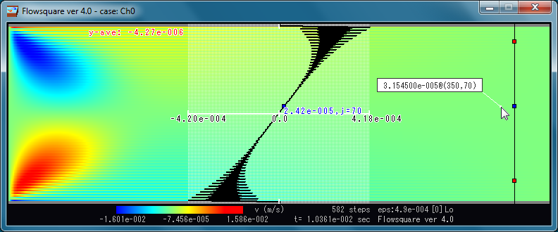
In the previous two lessons, we leant how to start simulation (Lesson 1.1), and some of display operations (Lesson 1.2). In Lesson 1.2, we also observed there are numerical oscillations in the velocity and vorticity fields (Figs. 9 and 10 of Lesson 1.2). In this lesson, we will learn how to set some of parameters in grid.txt for better accuracy and/or numerical stability.
Generally in CFD (Computational Fluid Dynamics), more simulation accuracy requires more computational resources (computational time, RAM, mode complicated codes, …). Also most of the time, we have to compromise simulation accuracy and computational time for numerical stability. Please bear in mind them and let’s move on.
Remove numerical wiggle
First, let’s consider the numerical oscillations we observed in Lesson 1.2. We start from the original grid.txt for the 2D Channel Flow case which can be downloaded from here. Open grid.txt in the main directly. As explained in Lesson 1.1, grid.txt specifies numerical parameters. All lines except line separators consist of 3 blocks. For example, after the second line separator, you see this:
01:cmode 0 // Simulation mode, ....
The first block (01:cmode) denotes a name of each parameters (often similar name to the notation used in the Users’ Guide). The second block (“0” in above example) is the number you specify for each parameter. Then the third block (// Simulation mode, …) is just a comment, and nothing to do with the simulation results. These three blocks have to be separated by space(s).
Please locate the following lines:
02:nx         384  // No. grid points in x

03:ny         128  // No. grid points in y

04:lx       0.015  // Domain x-size

05:ly       0.005  // Domain y-size
As the comments say, nx and ny are respectively number of grid points in x and y directions, and lx and ly are respectively the length in x and y directions (use SI units). Since Flowsquare solves flow field using Finite Difference Scheme, more number of grid points in a unit domain length means more accurate your simulation would be. However, more grid points massively increases the computational time, so you have to balance between the resolution and computational time. Also, except for special cases, the grid densities (lx/nx and ly/ny) in x and y direction should be equal.
Now, we have following lines in grid.txt.
10:nfil         0  // Interval time steps for filtering

11:wfil         0  // Relaxation parameter for filtering
These lines are directly related to the current problem — unphysical oscillation. Filtering means you add a viscosity to your flow so that tiny wiggles, which are too small to be physical, disappear. Let’s change the above lines to:
10:nfil         1  // Interval time steps for filtering

11:wfil         1  // Relaxation parameter for filtering
and start the simulation. Let’s use “Ch0_filter” as the simulation case name. At around 600 time steps (approx 1 minute simulation), halt the simulation and display a cross sectional graph of v (vertical velocity component) field, just like the one shown in Figure 9 in Lesson 1.2. However this time, the wiggle disappears and the v field would be smooth like Fig. 1 shown below.
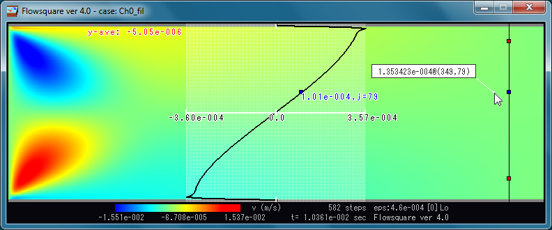
Figure 1: v (vertical velocity component) field after using filtering option.
Generally, you will need to use filtering for most of simulations. However, using wfil = 1 can sometimes be too much and it may result in a fluid like ketchup. I recommend you use wfil as small as possible (I would use 0.01–0.1).
Enhance accuracy
You may find following line specifying a numerical scheme you use in the simulation:
09:iorder 0 // 0: low order, 1: high order, ....
You can use a number from 0 to 3 for iorder to choose from numerical schemes, and each number means:
- iorder=0: Low order scheme (2nd order difference, 1st order time integral)
- iorder=1: High order scheme (4th order difference, 3rd order time integral)
- iorder=2: 2nd order difference and Lax-Wendroff time marching (2nd order)
- iorder=3: 4th order difference and Lax-Wendroff time marching (2nd order)
Here, let’s specify 1 for iorder (as follows), which means we will use a high order scheme to enhance simulation accuracy.
09:iorder 1 // 0: low order, 1: high order, ....
Also, since we want to simulate as accurately as possible, remove all the additional viscosity by turning off the filtering as this:
10:nfil         0  // Interval time steps for filtering

11:wfil         0  // Relaxation parameter for filtering
Now, we are ready to start high accuracy simulation of the 2D channel flow. This time, computational time can be much longer (approx 3-5 times). You may halt the simulation and check if there are numerical wiggles (hopefully not!). Let’s name the high order simulation as “Ch1”, and simulate the flow using the high accuracy scheme until 4000 time steps. Next, we will compare the low and high order simulation results by using post-analysis mode. Thanks for reading!