When the solution diverges…
When the solution numerically diverges and you can no longer continue simulation, check and try to change items as follows. Note the details of following parameters can be found in the Users’ Guide.
- Is the domain size same as the size of bc.bmp?
The domain size (nx, ny in grid points) defined in grid.txt should be identical to the pixel size of bc.bmp. Note that Flowsquare automatically interpolates the figure if these sizes are not equal, but this function sometimes does not work perfectly. - Is spatial resolution enough?
As said in Lesson 2.1, pixel size of bc.bmp also defines the spatial resolution of computational domain (note that the domain is discretised into nxXny mesh points. see Lesson 0). Thus, bc.bmp needs to have sufficient pixel density to represent the aerodynamic object in the figure.[EXAMPLE]
Suppose you want to simulate a flow field around two-dimensional plate. The left figure represents this plate with 1 pixel thickness. This obviously is not adequate for CFD since the flow wrapping around the tips of the plate cannot be resolved with 1 mesh point. Thus, the plate should be illustrated using several pixels such way in the right figure, and bc.bmp needs to be changed accordingly.
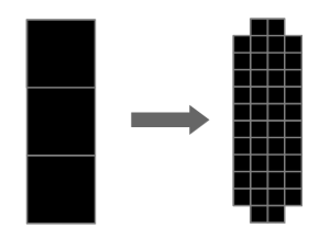
Left: bad example. Right: good example. One black square represents one pixel in the bmp file.
- Increase cflfac
Cflfac in grid.txt directly related to the reciprocal of the time stepping (delta t). Thus, the time resolution becomes better with an increase of cflfac. The optimal value is around 10–20 for most of the cases, but larger value may be used for more complicated cases. - Reduce nfil (close) to 1
Nfil in grid.txt defines interval time steps of spatial filtering operation. By setting this to be 1, the solution is spatial filtered in every timestep, which may result a stable solution. Note nfil is integer. To turn off this operation, put 0. - Increase wfil
Wfil in grid.txt defines the amount of filtered solution to be added to the raw solution. Usually 0.05–0.2 are optimal, although smaller value is sometimes theoretically desirable. The maximum value is 1. - Decrease omega
Omega in grid.txt defines a relaxation parameter for Poisson’s equation, and is related to cmode=0, 1 and 2. Although, Omega=1.8 is optimal for most of the cases, lowering this value may be required for some of complicated flow configurations.
