In the previous lesson, we’ve learnt how to start simulation using the pre-set channel flow case. In this page, we will learn some of the functions you can use during simulations. In the simulation of a 2D channel flow, you see a window displaying u as in Fig. 1.
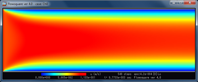
Figure 1: Simulation window during 2D channel flow (original bc.bmp and grid.txt).
This display is boring. So let’s make it a bit more interesting and more informative. Hit [Ctrl] + T while the simulation window is active, and you will see something like this on the top-left corner of the simulation window as in Fig. 2. This shows the computational time per each time step, and physical time increment (time stepping) per time step. In the case of Fig. 2, it takes 49 (ms) (milliseconds) to compute one time step, and the physical time increases by 0.0178 (ms) at every time step. Note that the computational time varies depending on the computer you use. I use a laptop fitted with Core i5-2400M CPU@2.50GHz on Windows 7 (They do a decent job!). To turn off, press [Ctrl] + T once again.
![Figure 2: [Ctrl] + T displays the computational time per time step and physical time increment. To turn off, [Ctrl] + T once again.](http://flowsquare.com/wp-content/uploads/2013/12/Window_Ch0_2.png)
Figure 2: [Ctrl] + T displays the computational time per time step and physical time increment. To turn off, [Ctrl] + T once again.
Only one quantity (u) may not give a good image of the flow field to you. Press ↑ (up arrow key), and you will see velocity vectors overlaid on the u field as in Fig. 3. Now, it may be clearer to you that the fluid flows from left to right. The colour of the vector, number of vectors, pixel size of arrows can be adjusted by users by editing grid.txt, by using keyboard short cut keys, or they are determined automatically. To turn off the vector display from the simulation window, press ↓ (down arrow key).
![Figure 3: [↑] (up arrow key) displays velocity vectors overlaid on the shown field.](http://flowsquare.com/wp-content/uploads/2013/12/Window_Ch0_3.png)
Figure 3: ↑ (up arrow key) displays velocity vectors overlaid on the shown field.
Sometimes, even during the simulation, you may need to examine your instantaneous flow field. In such a case, you want to halt the simulation. Press [ESC] while your simulation is going and you will be asked to choose a option as in Fig. 4. Then press [Enter] to continue the simulation, press Q to end the current case, or press any other keys (except [ESC]) to start an analysis on the current instantaneous flow field. Here, let’s press any other keys (except [ESC]), and see what your 2D channel flow field is like.
![Figure 4: Press [ESC] key during the simulation and you will be asked to choose a option.](http://flowsquare.com/wp-content/uploads/2013/12/Window_Ch0_ESC.png)
Figure 4: Press [ESC] key during the simulation and you will be asked to choose a option.
Analysis mode
If you choose analysis mode by hitting one of the keys on the display shown in Fig. 4, you will see a display something similar to Fig. 5 subsequently. In this mode, you can see numbers following the mouse cursor inside the computational domain. These numbers show local value at the cursor location of shown field. In the case of Fig. 5, numbers are something like “1.118477e-001@(122,60)” overlaid on the u velocity field. This means at (i, j)=(122, 60), u=0.1118477 (m/s). Here, i and j means location of the cell. For the present channel flow case, 1<i<384 (horizontal axis) and 1<j<128 (vertical axis). Move around the mouse cursor to examine your u field in detail.
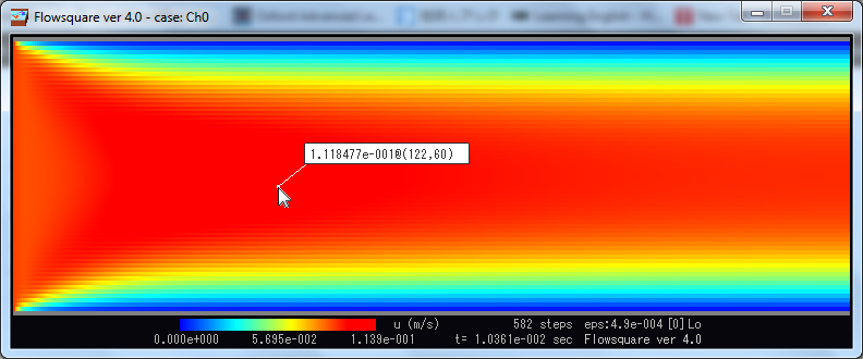
Figure 5: Analysis mode window.
Display a Graph
In the analysis mode window, click the left button of the mouse (left-click) and you will see a tiny red square appears on the location of your cursor. Then, move your mouse a little (or more) and left-click again. Now you will see a cross-sectional graph of u field along the black line connecting these two tiny red squares (Figs. 6–8). To turn off the graph display, left-click once again (but you are not required to do so here).

Figure 6: Click the left button of the mouse (left-click) and you will see a tiny red square appears on the location of your cursor.
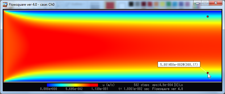
Figure 7: Move your mouse a little (or more) and left-click again.
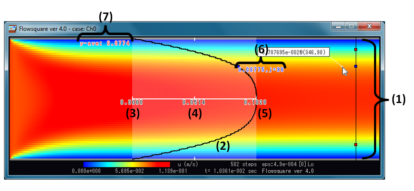
Figure 8: Now you will see a graph of u field along the black line connecting these two tiny red squares.
Note that you can also construct a cross-sectional graph along x (horizontal) axis. The things shown in the graph window are explained in below (please refer to the number in Fig. 8.).
- The black line stretching to y(vertical) direction connects the two tiny red squares you made (by left-clicks). The data for the graph is extracted along this black line (cross-section).
- The graph of the cross-section
- The minimum value in the cross-section
- The middle value in the cross-section
- The maximum value of the cross-section
- The local value at the location of the tiny blue square on the cross-section. The blue square moves following mouse’s y location, which is also shown in the graph.
- Cross-sectional average of the shown field except for the wall boundary regions.
–
Change displayed field
Maybe you are a bit bored with the u field. Let’s display another field — density, v, speed, vorticity, etc. To change displayed field, use following keys.
- rho (kg/m^3): 1
- u (m/s): 2
- v (m/s): 3
- spd (m/s): 4
- vort (1/s): 5
- temp (K): 6
- rate (kg/m^3s): 7
- c/xi: 8
- p-p0 (Pa): 9
- xi_air: [Shift]+8
- prs2(kg/m^3s^2): [Shift]+P
If you need to look up for what these characters (eg. rho (kg/m^3)) mean, go back to the previous post any time. Note that the graph and these keys can be used during the simulation as well (although your simulation speed becomes a bit slower). Here, let’s display v (vertical velocity component) field (by hitting 3) as in Fig. 9. Now, both colour and graph shows v field. As you can see, there are a lot of numerical oscillations (we will learn how to minimise them later). Now press 2 to get back to u field and left-click to turn off the graph (and you see something like Fig. 5).
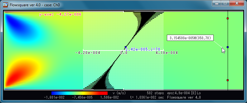
Figure 9: Display v (vertical velocity component) field by pressing 3.
–
Display contour lines
There are one more feature I have to explain . Press right button (right-click) of your mouse inside the computational domain. You should see that a contour line appeared at the level your mouse cursor are, as in Fig. 10. The tiny box with a number on the top-left corner displayed for 1 second after you add the contour line shows how many contour lines you used so far (contour counter). You can add more contour lines (up to 50) just by right-clicking on your mouse. To remove the last contour line you have made, press [Space] key, and the contour counter decreases by 1. To remove all of the contour lines, press [Delete] key, and the contour counter is reset to zero.
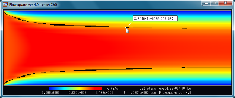
Figure 10: Right-click displays contour line(s) of the field.
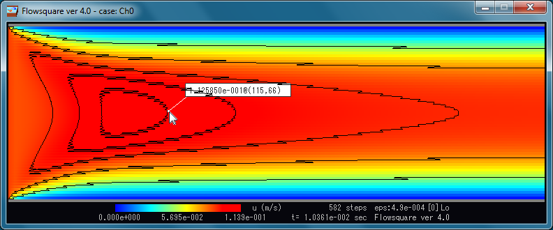
Figure 11: More and more contour lines (up to 50) if you right-click more. (Hahaha, numerical oscillation is obvious.)
If you have played a lot with your current instantaneous flow field, let’s resume the simulation by pressing [ESC] key to get out from the analysis mode. You leant a lot, but these are only part of what Flowsquare does. We will learn more soon. Thanks for reading.