In this page, we will learn a series of procedures required to simulate flows with Flowsquare using an example numerical setting. At this moment, you don’t need to read through or understand what is written in the Users’ Guide. Also, don’t worry if you encounter some words which you don’t understand. You will understand them eventually.
Continue reading
Monthly Archives: November 2013
Lesson 0 — Before You Start…
Before you start (or after you started), it’s good idea to know a little bit of basics of how we simulate a flow field. Suppose Fig. 1 is the flow field we want to solve.
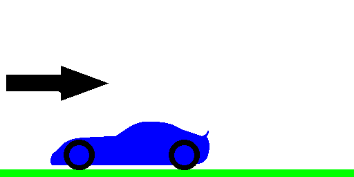
Figure 1: Flow field we want to solve.
There are 3 steps to simulate the flow.
First, we discretise the field into NX x NY mesh points as in Fig. 2 (NX and NY are numbers of mesh points in horizontal and vertical directions).
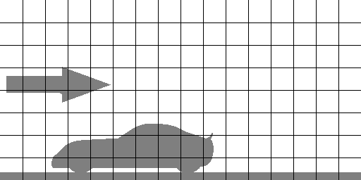
Figure 2: First we discretise flow field into nx x ny mesh points.
Second, we calculate many Many MANY equations on each mesh point (in space) to obtain the instantaneous solution. The equations are explained in the Users’ Guide.
Third, we advance the solution little (dt) by little (dt) in time to obtain temporal change of the flow. Here, dt is the physical time increment per time step and typically this has an order of microseconds.
This is how Flowsquare simulates flows. Easy peasy!