In this page, we will learn a series of procedures required to simulate flows with Flowsquare using an example numerical setting. At this moment, you don’t need to read through or understand what is written in the Users’ Guide. Also, don’t worry if you encounter some words which you don’t understand. You will understand them eventually.
Inside the Box (folder)
I am sure you have already downloaded and uncompressed the software (if not, see DOWNLOAD). Make sure there are flowsquare.exe, bc.bmp and grid.txt in the main directory (folder). They have important roles as follows.
- flowsquare.exe: The software
- bc.bmp: A bitmap image that contains boundary condition of the simulation
- grid.txt: A text file that contains all the simulation parameters
These files are initially set up for a simulation of 2D channel flow, so you don’t need to change them for now. Additionally, you may use following input files depending on your simulation cases (but we use the above three files only in this page!).
- ic.bmp: A bitmap image that contains initial condition of the simulation
- bg.bmp: A bitmap image for the background of the simulation domain
Remember that bc.bmp, grid.txt, ic,bmp (optional) and bg.bmp (optional) are the input files for simulations, and every time you start a simulation these files are read from the main directory.
Two-dimensional channel flow
We will simulate a two-dimensional channel flow using the default input files. A two-dimensional channel flow is a flow where fluid flows between two parallel walls. The schematic illustration of the simulation flow field is shown in Fig. 1 below.
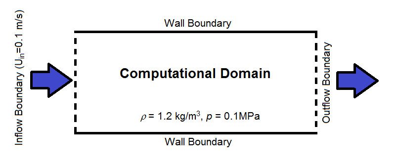
Figure 1: Numerical configuration
Run the simulation
Double click flowsquare.exe to run your first fluid flow simulation. Figure 2 is what you see. Let us skip this reminder by hitting Enter key. You will be reminded every time you start a simulation, or you could donate to receive a Donation License or to request a Student license later to obtain a password and unlock the software. Note that you can use Flowsquare’s maximum computation speed once you unlock the software with the password. See License Types.

Figure 2: Skip this page or unlock the software.
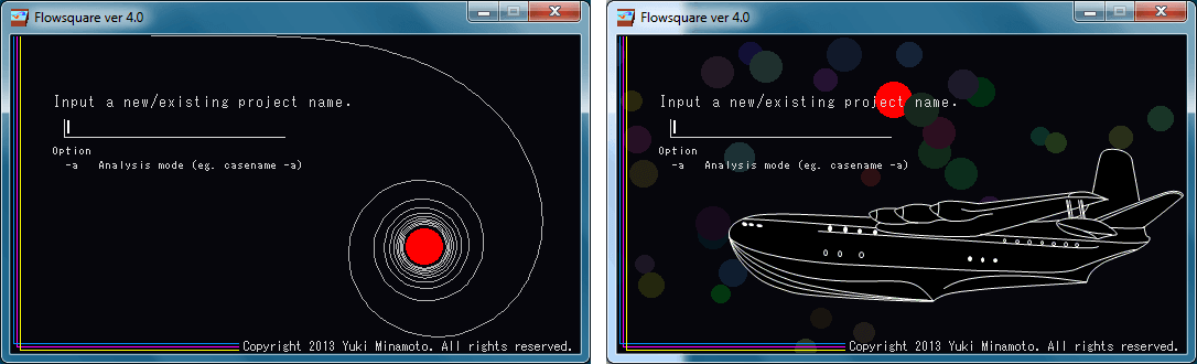
Figure 3: (Step 1) Enter your simulation case name.
Figure 3 shows what you see after skipping the donation reminder (note you will see a different window design randomly). Here, you need to decide your simulation case name, put it in the box and then hit the Enter key. You can use any name you want, but here let’s use “Ch0” for the case.
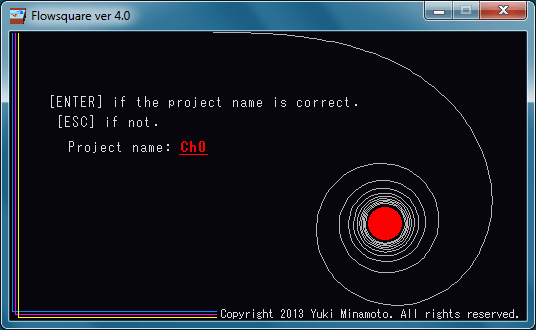
Figure 4: (Step 2) Confirm the case name and then hit Enter key.
Now, you can see a window something like Fig. 4. If you don’t like the case name, hit ESC key to go back to the previous window. If you are happy with the case name, let’s hit Enter key and simulation will begin subsequently.
Explanation of the simulation display
If you run your first simulation using the original files, you will see something similar to Fig. 5. The shown field is u, which is x-component velocity, and the fluid flows from left to right. There are some numbers and characters that mean something. Descriptions are as follows (refer to the numbers in Fig. 5), but please don’t worry if you don’t understand some of the words for now.
- Current case name
- Color bar of current color map. The left, middle and right numbers are respectively the minimum, middle, and maximum values of displayed field.
- Name of the displayed field. There are:
- rho (kg/m^3): Mixture density
- u (m/s): Velocity component in x-direction
- v (m/s): Velocity component in x-direction
- spd (m/s): Velocity magnitude (sqrt(u^2+v^2))
- vort (1/s): Vorticity
- temp (K): Temperature (for Premixed/Non-premixed cases)
- rate (kg/m^3s): Reaction rate (for Premixed cases)
- Ma: Mach number (for Sub/supersonic cases)
- c/xi: Scalar / progress variable / mixture fraction (for some of Non-reactive, and Premixed/Non-premixed cases)
- p-p0 (Pa): Pressure – reference pressure, pres0 in grid.txt
- xi_air: Mixture fraction between progress variable and pure air (for some of Premixed cases)
- R/rho (J/kg): total energy/density (for Subsonic/supersonic cases)
- prs2(kg/m^3s^2): (du/dx+dv/dy)/dt — a term appears in the Poisson’s equation (for all cases except Subsonic/supersonic cases)
- Physical time (seconds)
- Current time step
- Convergence limit of iteration calculation for Poisson’s equation
- Current simulation mode. There are four modes and specified in grid.txt.
- [0]: Non-reactive, incompressible flows
- [1]: Premixed reactive flows
- [2]: Non-premixed reactive flows
- [3]: Subsonic/supersonic inviscid flows
- Current numerical scheme. There are four sets of schemes available and specified in grid.txt.
- Lo: 2nd order Central Finite Difference and Euler (1st order) methods
- Hi: 4th order Central Finite Difference and 3rd order Runge-Kutta methods
- lw: 2nd order Central Finite Difference and Lax-Wendroff (midpoint) methods
- LW: 4th order Central Finite Difference and Lax-Wendroff (midpoint) methods

Figure 5: Simulation display.
If you use the default bc.bmp and grid.txt, the simulation will stop at 4000th time step and the window goes back to Figs. 2 or 3. Go to the directory having the case name you just did (“Ch0” if you followed the above instruction), and check if there are three sub-folders: bkup, dump, and figs. These folders contain:
- bkup: Backup data of the simulation input files; grid.txt, bc.bmp, ic.bmp (optional) and bg.bmp (optional)
- dump: Dump data (or restart data or simulation result data, but all the same!)
- figs: Output figures
For the default setting, dump data is saved once in every 2000 time steps, and a figure is generated once in every 200 time steps (you can know the generated time step from the data/figure name). Are figure meaningful to you or not? Soon, you will be able to know a lot from the figure. Thanks for reading!