In Lessons 1.1-1.3, we learnt how to run simulations and the meanings of some of parameters specified in grid.txt. We also run simulations using the low order scheme (case name: Ch0) and the high order scheme (case name: Ch1). In this lesson, we will compare these two results by using post-analysis mode included in Flowsquare.
Using Post-analysis mode
If you followed Lessons 1.1–1.3, you have (at least) results of two simulations; “Ch0” and “Ch1”. First, run Flowsquare.exe and type “Ch0 -a” in the case name field (Fig. 1) and hit Enter. Here, ” -a” (“space“, “–” and “a“) is the option command for Post-analysis mode, and we will use this mode for Ch0 case. In Post-analysis mode, all the input files such as grid.txt and bc.bmp are read from the backup folder (bkup under the case-name folder).

Figure 1: Enter “Ch0 -a” as case name.
Now, you see the simulation results of Ch0 case as in Fig. 2.
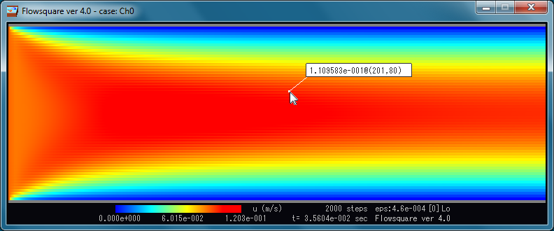
Figure 2: Post-analysis window.
Using Page up (PGUP) and Page down (PGDN) keys, you can change the time step of displayed results. Note the result of the time step you want to display has to be saved during the simulation by setting nfile parameter in grid.txt. For the default setting you have instantaneous results at 0, 2000, 4000th time step. Let’s display 4000 time step results by using the PGUP key. You may draw a cross sectional graph. For the Ch0 case, the result at 4000th tims step may look something like this (Fig. 3):
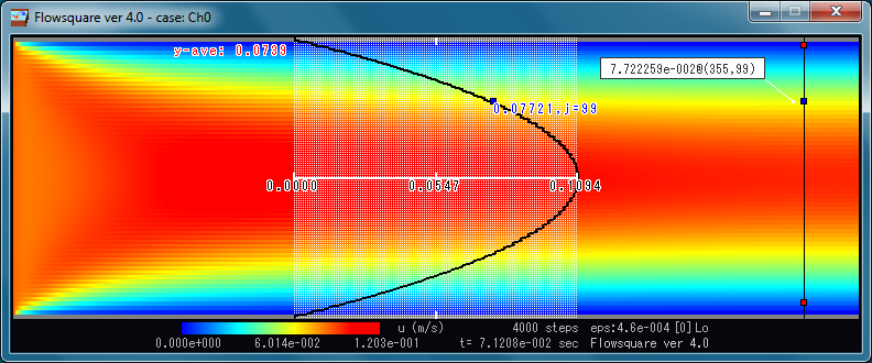
Figure 3: Ch0 case (low order), u field, ts(time step)=4000, location of the graph is i=360.
Comparison between low and high order results
In the same way, you can display Ch1 (high order results) and you may see this (Fig. 4):
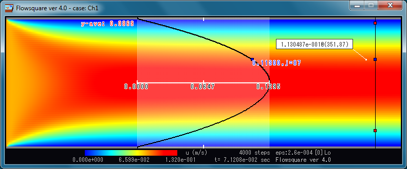
Figure 4: Ch1 case (high order), u field, ts(time step)=4000, location of the graph is i=360.
At the same physical time, under the same flow conditions, but clearly there are differences between Ch0 (low order) and Ch1 (high order) cases. So which is correct? For 2D channel flow configuration, you can obtain the analytical solution. According to the solution, the maximum u velocity is 1.5 times of cross sectional average of u velocity. Also, the u variation should be parabolic.
For Ch0 case (low order), the maximum u is 0.1094 (m/s) and the cross-sectional average is 0.0739 (m/s) as in Fig. 3. The ratio of the two is 0.1094/0.0739=1.480, which means 98.7% of the theoretical value. It’s good!
For Ch1 case (high order), the maximum u is 0.1295 (m/s) and the cross-sectional average is 0.0869 (m/s) as in Fig. 4. The ratio of the two is 0.1295/0.0869=1.490, which means 99.3% of the theoretical value. It’s better!
Also, the low order scheme is usually more dissipative, and this is the main reason why average velocity is smaller in Ch0 (low) than in Ch1 (high). For these reasons, (as we expect) the high order scheme wins!
However, computation with a low order scheme is much quicker. You have to balance these factors when you determine the simulation conditions and methods. There are loads more to explore, which we will learn soon. Thanks for reading.