There are many keyboard shortcuts used in Flowsquare. Note these keyboard operations are detected once in a transition between displays from an old time step (eg. n-1) to a new time step (eg. n), and the operation is reflected in display for the next time step (eg. n+1). Continue reading →

All parameters considered for solving the governing equations in Users’ Guide are specified in grid.txt. In grid.txt, all lines except line separators consist of 3 blocks. For example, first three lines of grid.txt look something like this: Continue reading →

Initial conditions (I.C.) are as important as boundary conditions. In Flowsquare, however, initial conditions are set according to the B.C. set in bc.bmp and the initial values specified as following variables in grid.txt. Continue reading →

In Lessons 1.1-1.3, we learnt how to run simulations and the meanings of some of parameters specified in grid.txt. We also run simulations using the low order scheme (case name: Ch0) and the high order scheme (case name: Ch1). In this lesson, we will compare these two results by using post-analysis mode included in Flowsquare.
Continue reading →

In the previous two lessons, we leant how to start simulation (Lesson 1.1), and some of display operations (Lesson 1.2). In Lesson 1.2, we also observed there are numerical oscillations in the velocity and vorticity fields (Figs. 9 and 10 of Lesson 1.2). In this lesson, we will learn how to set some of parameters in grid.txt for better accuracy and/or numerical stability.
Continue reading →

In the previous lesson, we’ve learnt how to start simulation using the pre-set channel flow case. In this page, we will learn some of the functions you can use during simulations. In the simulation of a 2D channel flow, you see a window displaying u as in Fig. 1.
Continue reading →

In this page, we will learn a series of procedures required to simulate flows with Flowsquare using an example numerical setting. At this moment, you don’t need to read through or understand what is written in the Users’ Guide. Also, don’t worry if you encounter some words which you don’t understand. You will understand them eventually.
Continue reading →

Before you start (or after you started), it’s good idea to know a little bit of basics of how we simulate a flow field. Suppose Fig. 1 is the flow field we want to solve.

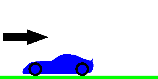
Figure 1: Flow field we want to solve.

There are 3 steps to simulate the flow.

First, we discretise the field into NX x NY mesh points as in Fig. 2 (NX and NY are numbers of mesh points in horizontal and vertical directions).

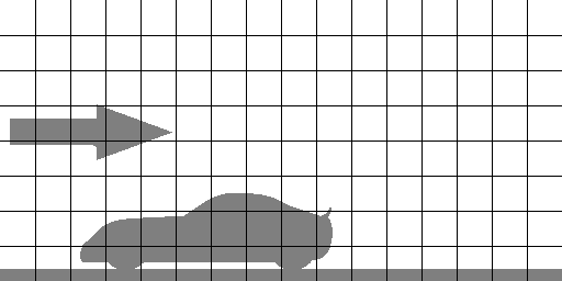
Figure 2: First we discretise flow field into nx x ny mesh points.

Second, we calculate many Many MANY equations on each mesh point (in space) to obtain the instantaneous solution. The equations are explained in the Users’ Guide.

Third, we advance the solution little (dt) by little (dt) in time to obtain temporal change of the flow. Here, dt is the physical time increment per time step and typically this has an order of microseconds.

This is how Flowsquare simulates flows. Easy peasy!